The screenshots come from Excel in Portuguese.
What it’s for
A SUMIFS with three criteria returns a number, and the next question comes right after: which rows of the data went into it? And when the result looks low or comes out zero, which criterion left a row out? Until now, the answer meant filtering the data, checking row by row and clearing the filter.
With the criteria highlight, the sheet itself answers: with the focus on a SUMIFS in the Inspect, each criteria column shows the cells that meet it, and the sum column shows what goes into the result. Excel itself decides the color, with the SUMIFS rule: wildcards, dates and <> are highlighted the way the formula counts them.
How to use it
-
Turn the highlight on once: in Excel, the Lubre Sheets Settings button (Home tab), Appearance tab, Highlight what the Inspect traced option.

-
Select the cell with the SUMIFS, open the Inspect (Alt+↑; Option+↑ on Mac) and press ↓ down to the SUMIFS row. The sheet gets three shades of the same color: light on the range, medium on the cells that meet that column’s criterion and strong on what goes into the result. A row that was left out shows, in the row itself, which criterion excluded it: it’s the column that isn’t in the medium shade.
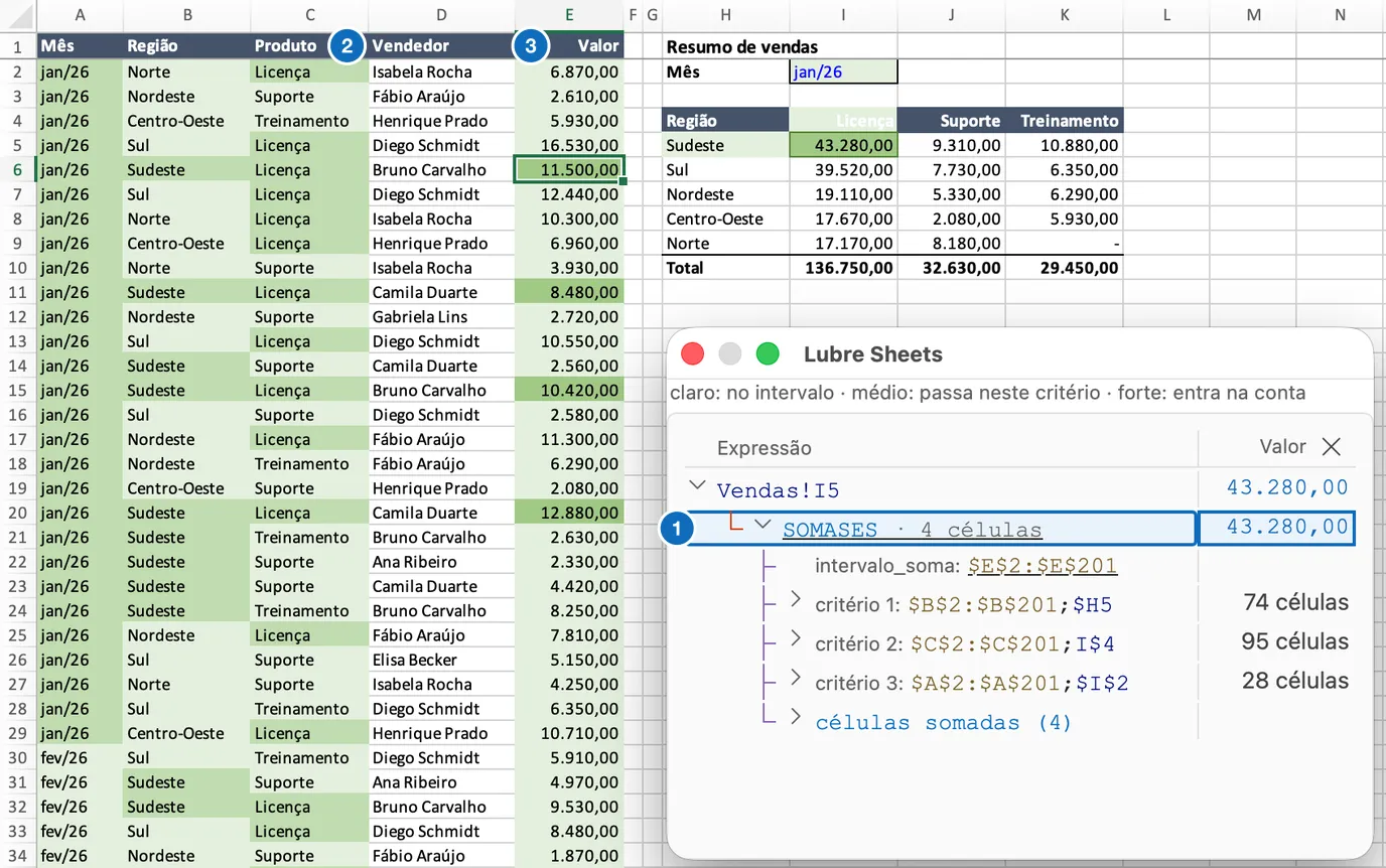
-
Read the counts in the tree. Each criterion shows how many cells meet it, and the SUMIFS row shows how many go into the result. When the result is zero, the tree points to the reason: no cells on the criterion nobody meets, or 0 with previous on the criterion that zeroes the count together with the ones above. In the example, “Norte” sold “Treinamento” during the half-year, but not in January.
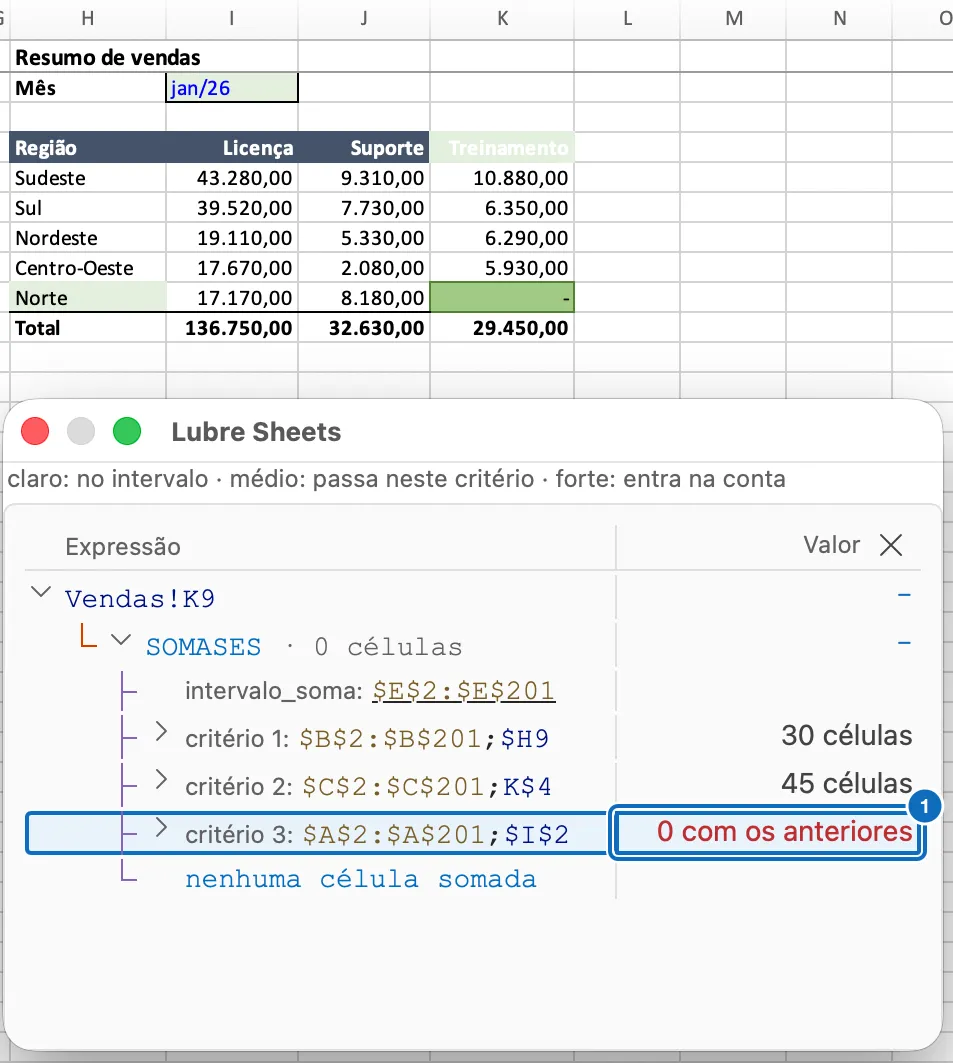
The color stays while you move through the criteria of the same SUMIFS. Ctrl+Shift+H (Control+Shift+H on Mac) turns the highlight on and off without leaving the Inspect. Click the sheet or close the Inspect and the color goes away.
Details
Which functions does it work with?
SUMIFS, SUMIF, COUNTIFS, COUNTIF, AVERAGEIFS, AVERAGEIF, MAXIFS and MINIFS, including inside a larger formula. In COUNTIFS, only the criteria columns are highlighted; in MAXIFS and MINIFS, the strong shade marks only the winning cell. It works with direct ranges ($E$2:$E$201), whole columns or defined names, and with data on another sheet: the Inspect takes you there.
What do I need?
An up-to-date Microsoft 365 (Windows 2509, Mac 16.100 or Excel on the web) and the highlight turned on in the Appearance tab (it’s off by default), in one of six colors. The counts in the tree show up even with the highlight off.
What changes in the file?
While it’s showing, the color is written to the file, on top of the cells: fill, font and borders don’t change. So when you close the file, Excel may ask you to save even if you only looked; the content is unchanged. If Excel crashes with the color on screen, the Remove Lubre highlights button in the Appearance tab clears it.
What’s not covered yet?
Table references (Table1[Amount]) aren’t highlighted yet. When something can’t be highlighted (array criteria, ranges in another file, ranges of different sizes or a criterion that returns an error), the Inspect window says why. It also warns when the data has hidden rows: they go into the result but aren’t visible. During co-authoring, in read-only files and on protected sheets, the highlight pauses.
Already a user? Close and reopen Excel to get the update.